net = pyscan.my_sample(core_set_pts2017, 200) + pyscan.my_sample(core_set_pts2010, 200)
disc_f = pyscan.DISC
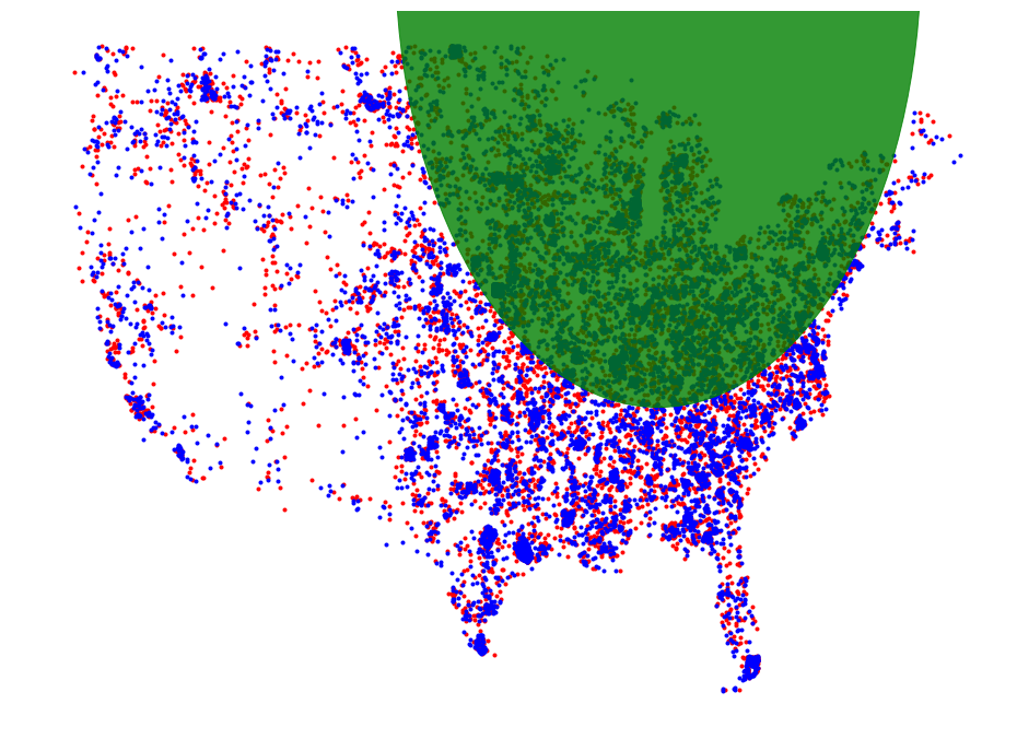
disk, d_val = pyscan.max_disk_scale(net,
[pyscan.WPoint(1.0, p[0], p[1], 1.0) for p in core_set_pts2017],
[pyscan.WPoint(1.0, p[0], p[1], 1.0) for p in core_set_pts2010],
1,
disc_f)
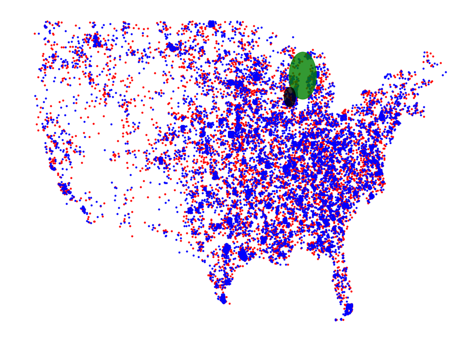
disk2, d_val = pyscan.max_disk_scale(net,
[pyscan.WPoint(1.0, p[0], p[1], 1.0) for p in core_set_pts2017],
[pyscan.WPoint(1.0, p[0], p[1], 1.0) for p in core_set_pts2010],
.5,
disc_f)
_, ax = plt.subplots(figsize=(16, 12))
plt.axis('off')
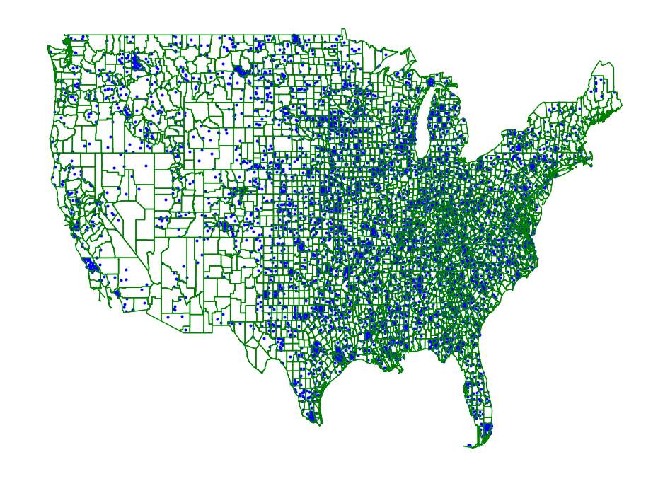
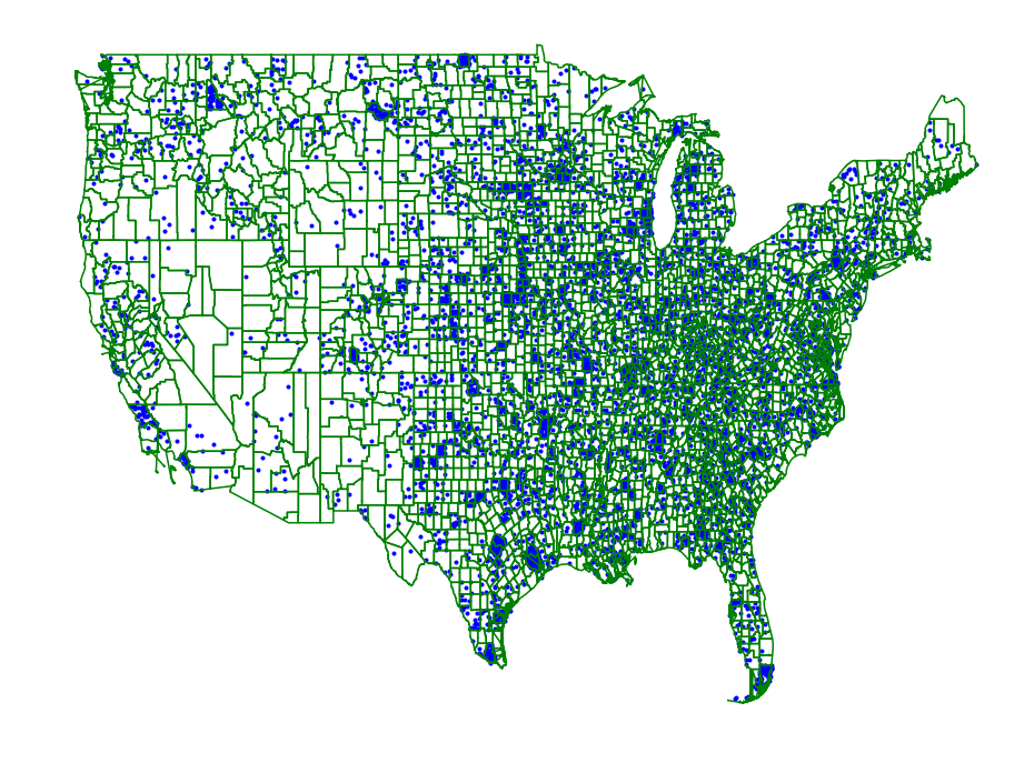
plot_points(ax, core_set_pts2010, "r")
plot_points(ax, core_set_pts2017, "b")
d = plt.Circle(disk.get_origin(), disk.get_radius(), color='g', alpha=.8)
ax.add_artist(d)
d = plt.Circle(disk2.get_origin(), disk2.get_radius(), color='k', alpha=.8)
ax.add_artist(d)
plt.show()
 pyscan
1.0
pyscan
1.0