Planting ExampleΒΆ

Below I create a code example where I plant a region containing 5% of the points and make this region anomalous. Inside of the region 80% of the points are from the red set while outside of the region 50% of the points are red. We would like to recover this planted region by using the max_halfplane scanning algorithm.

In [7]:
import pyscan
import matplotlib.pyplot as plt
import numpy as np
import random

def get_coord(i, lst):
    return [pt[i] for pt in lst]


# l = (a, b, c) where ax + by + c = 0 => (-ax -c) / b = y
def f(mr, x):
        l = mr.get_coords()
        return -(x * l[0] + l[2]) / l[1]

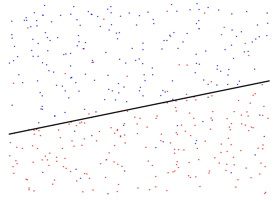
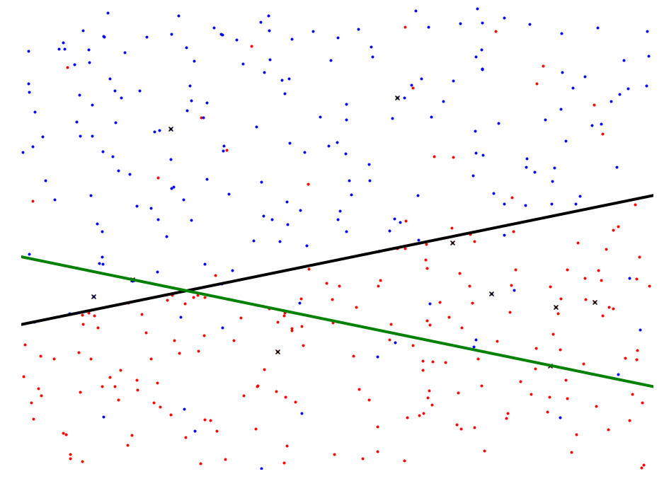
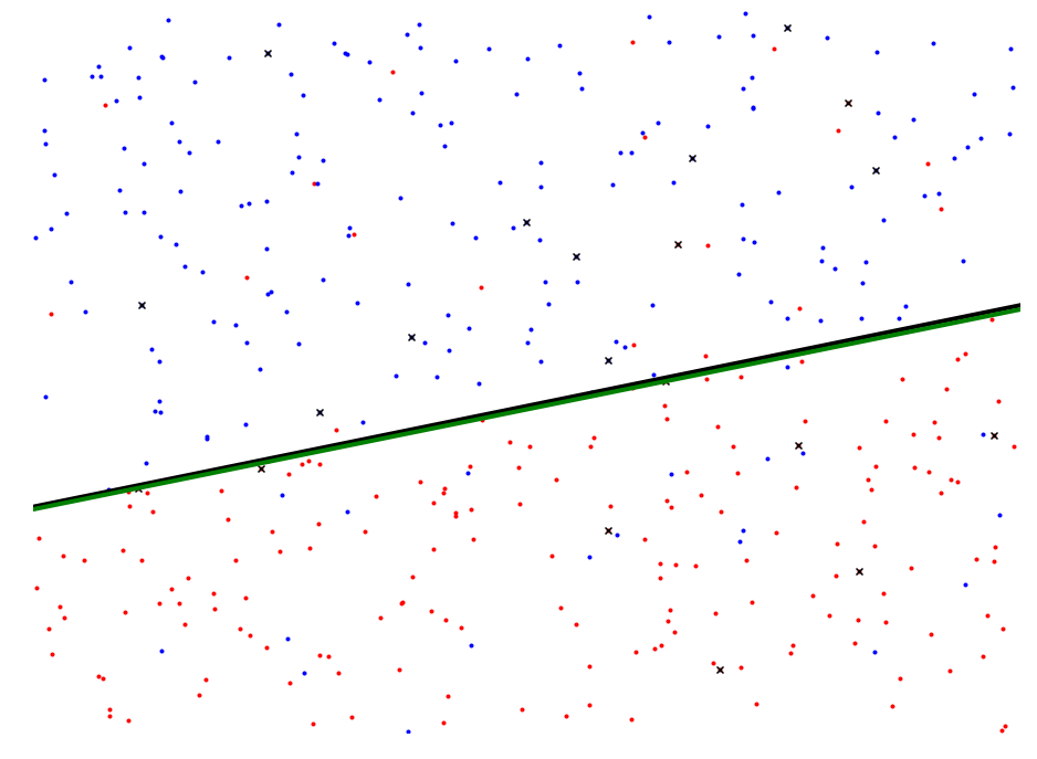
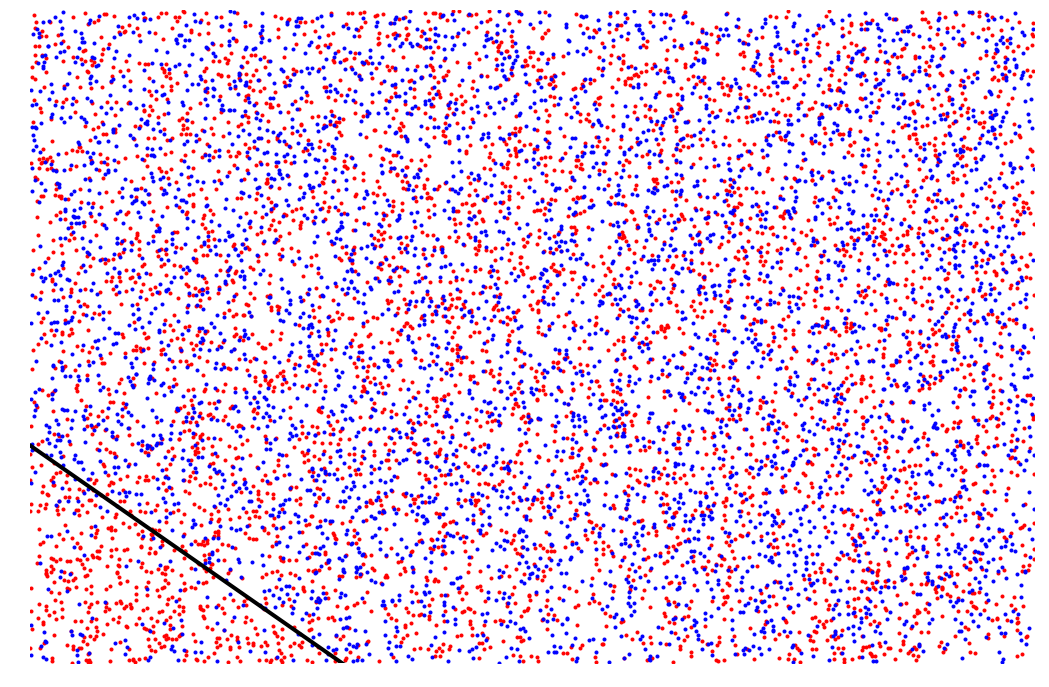
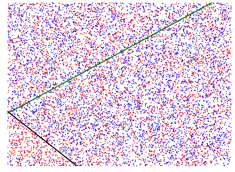
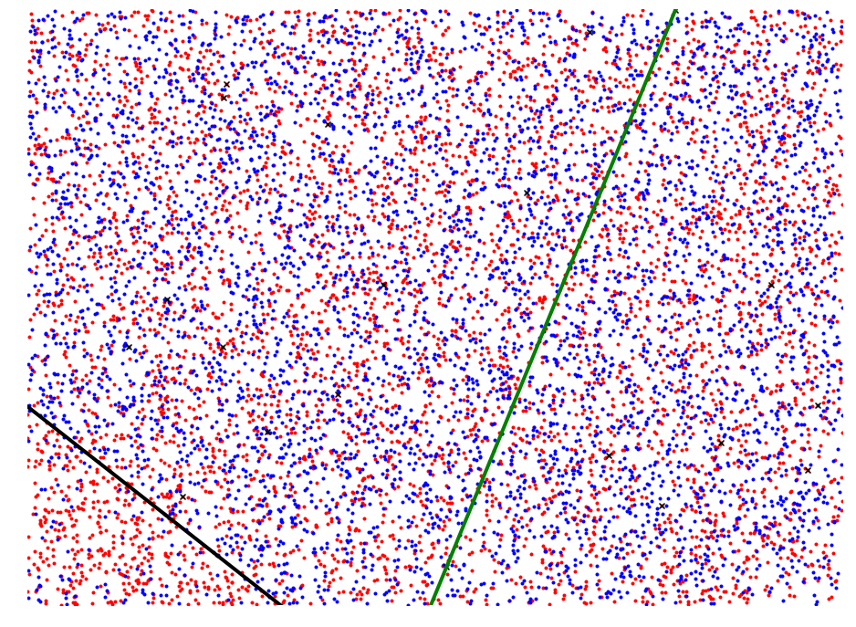
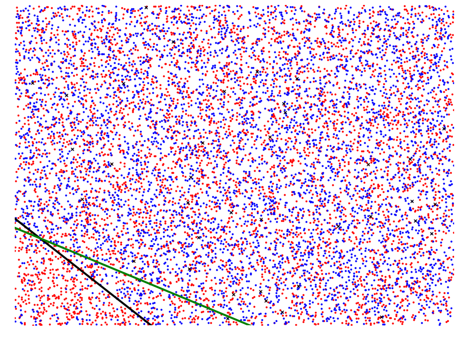
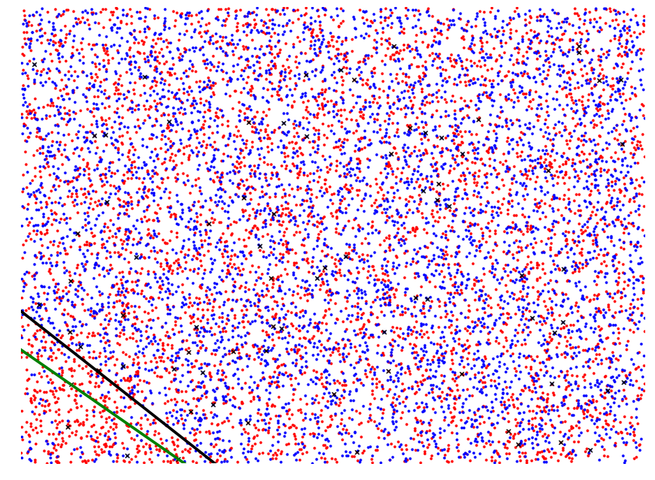
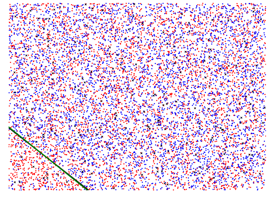
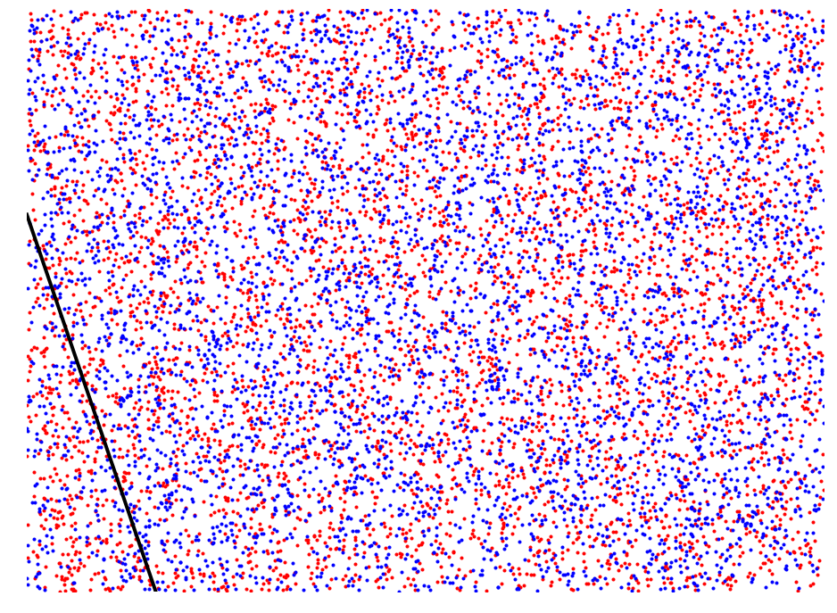
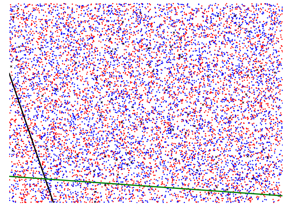
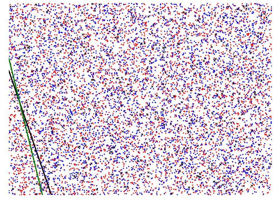
def plot_plane(red, blue, max_region, eps):

    n = np.rint(1 / eps)
    s = np.rint(1 / (2 * eps * eps))
    # create a region containing 5% of the points. Inside of this region points are more likely to be red.
    #print(get_coord(1, red))
    _, ax = plt.subplots(figsize=(16, 12))
    ax.scatter(get_coord(0, red), get_coord(1, red), marker=".", c="r")
    ax.scatter(get_coord(0, blue), get_coord(1, blue), marker=".", c="b")

    net = pyscan.my_sample(red, n) + pyscan.my_sample(blue, n)
    red_s = pyscan.my_sample(red, s)
    blue_s = pyscan.my_sample(blue, s)
    approx_region, _ = pyscan.max_halfplane(net, red_s, blue_s, pyscan.KULLDORF)

    ax.scatter(get_coord(0, net), get_coord(1, net), marker="x", c="k")
    ax.plot([0, 1], [f(max_region, 0), f(max_region, 1)], c="k", linewidth=4.0)
    ax.plot([0, 1], [f(approx_region, 0), f(approx_region, 1)], c="g", linewidth=4.0)
    plt.xlim([0, 1])
    plt.ylim([0, 1])
    plt.axis('off')
    plt.show()

We can plant a region that roughly cuts the point set in half and set two different halfs to be radically different. One side will have 90% percent red and the the other side 90% blue. The cutting region is in black.

In [8]:
pts = [pyscan.WPoint(1.0, random.random(), random.random(), 1.0) for i in range(400)]
red, blue, max_region = pyscan.plant_halfplane(pts, .5, .1, .9)
_, ax = plt.subplots(figsize=(16, 12))

ax.scatter(get_coord(0, red), get_coord(1, red), marker=".", c="r")
ax.scatter(get_coord(0, blue), get_coord(1, blue), marker=".", c="b")
ax.plot([0, 1], [f(max_region, 0), f(max_region, 1)], c="k", linewidth=4.0)
ax.set_xlim([0, 1])
ax.set_ylim([0, 1])
plt.axis('off')
plt.show()
../_images/examples_BasicExample_3_0.png

As we use a larger sample size we get better and better results. The algorithm will subsample the data based on an error parameter called \(\varepsilon\). There will be two samples uses in the algorithm one of size \(O(1/\varepsilon)\) and another of size \(O(1/\varepsilon^2)\). If we do not set \(\varepsilon\) to be small enough we will not recover the region. Below I steadily decrease \(\varepsilon\) and therefore increase the sample sizes. The small x markers define the regions that we scan. At first we will not recover the anomalous region.

In [11]:
plot_plane(red, blue, max_region, .2)
plot_plane(red, blue, max_region, .1)
../_images/examples_BasicExample_5_0.png
../_images/examples_BasicExample_5_1.png

In the above example we found the halfplane rather easily, but we can devise much more complicated situations where the region is much harder to recover.

In [14]:
# generate some random points
pts = [pyscan.WPoint(1.0, random.random(), random.random(), 1.0) for i in range(10000)]
red, blue, max_region = pyscan.plant_halfplane(pts, .05, .5, .8)
_, ax = plt.subplots(figsize=(18, 12))

ax.scatter(get_coord(0, red), get_coord(1, red), marker=".", c="r")
ax.scatter(get_coord(0, blue), get_coord(1, blue), marker=".", c="b")
ax.plot([0, 1], [f(max_region, 0), f(max_region, 1)], c="k", linewidth=4.0)
ax.set_xlim([0, 1])
ax.set_ylim([0, 1])
plt.axis('off')
plt.show()
../_images/examples_BasicExample_7_0.png

Now we are scanning a point set with 10000 points and the region is much smaller and less anomalous.

In [15]:
plot_plane(red, blue, max_region, .2)
plot_plane(red, blue, max_region, .1)
../_images/examples_BasicExample_9_0.png
../_images/examples_BasicExample_9_1.png
In [18]:
plot_plane(red, blue, max_region, .05)
../_images/examples_BasicExample_10_0.png

Around .025 we get start getting very close to recovering the region and at .01 we almost perfectly recover it.

In [19]:
plot_plane(red, blue, max_region, .025)
plot_plane(red, blue, max_region, .01)
../_images/examples_BasicExample_12_0.png
../_images/examples_BasicExample_12_1.png

We can plant a different where 60% of the points are from the anomalous red set and leave the baseline set at 50/50. This makes the region much harder to recover.

In [22]:
red, blue, max_region = pyscan.plant_halfplane(pts, .05, .5, .6)

_, ax = plt.subplots(figsize=(16, 12))
plt.scatter(get_coord(0, red), get_coord(1, red), marker=".", c="r")
plt.scatter(get_coord(0, blue), get_coord(1, blue), marker=".", c="b")
plt.plot([0, 1], [f(max_region, 0), f(max_region, 1)], c="k", linewidth=4.0)
plt.xlim([0, 1])
plt.ylim([0, 1])
plt.axis("off")
plt.show()
../_images/examples_BasicExample_14_0.png

We now fail to recover the region with the earlier parameters that were able to recover the region.

In [28]:
plot_plane(red, blue, max_region, .025)
../_images/examples_BasicExample_16_0.png

Increasing the error paramter even more allows us to again recover the region.

In [27]:
plot_plane(red, blue, max_region, .005)
../_images/examples_BasicExample_18_0.png