 pyscan
1.0
pyscan
1.0
- Installation
- API
- Examples
-
Site
- Installation
- Api
- Point
- Ranges
- Trajectory
- Trajectory Simplification
- Trajectories to Points
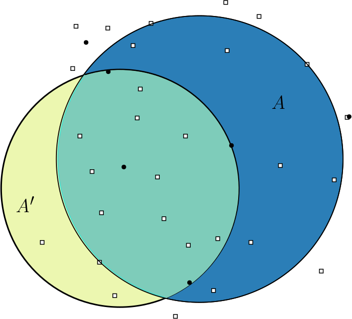
- Scanning
- Labeled Scanning
- Utility
- Examples
- Planting Example
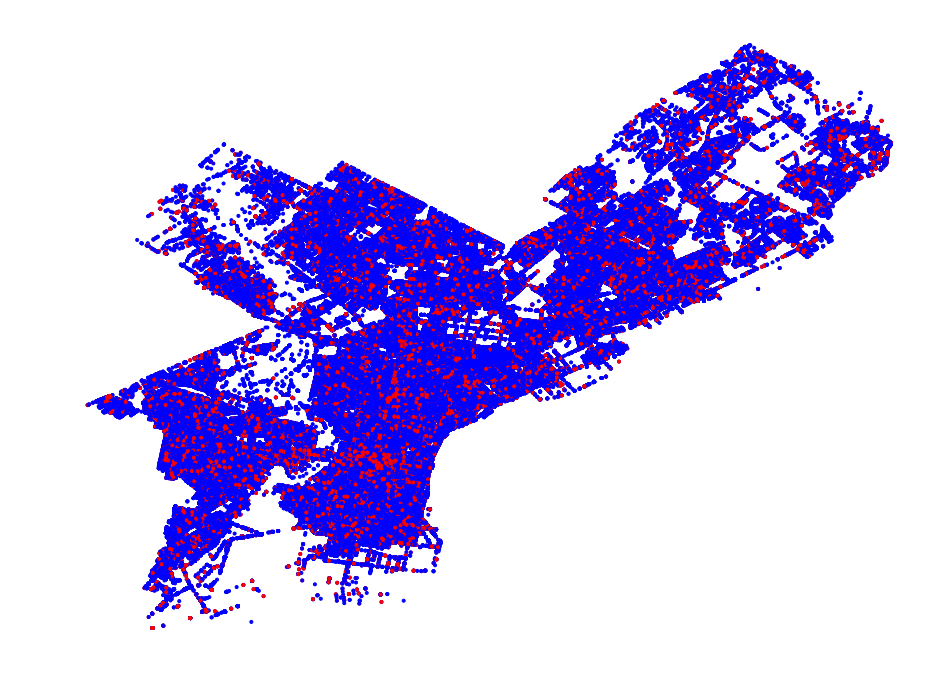
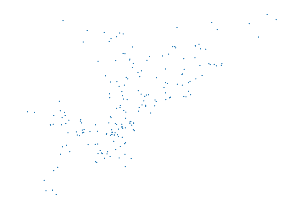
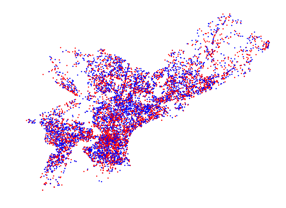
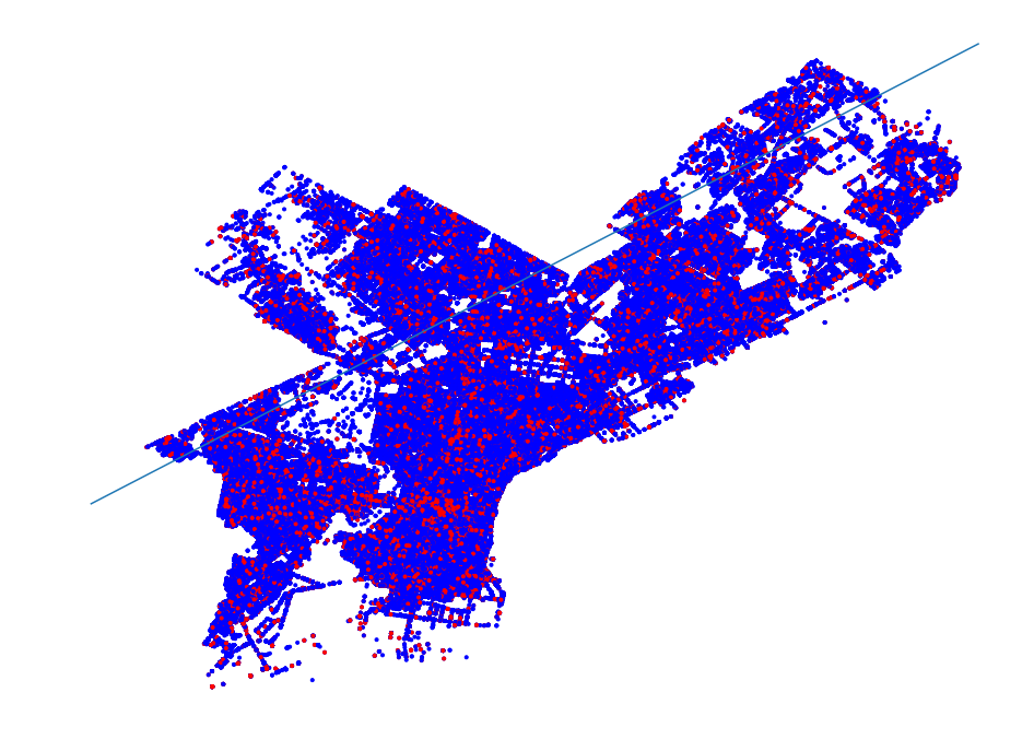
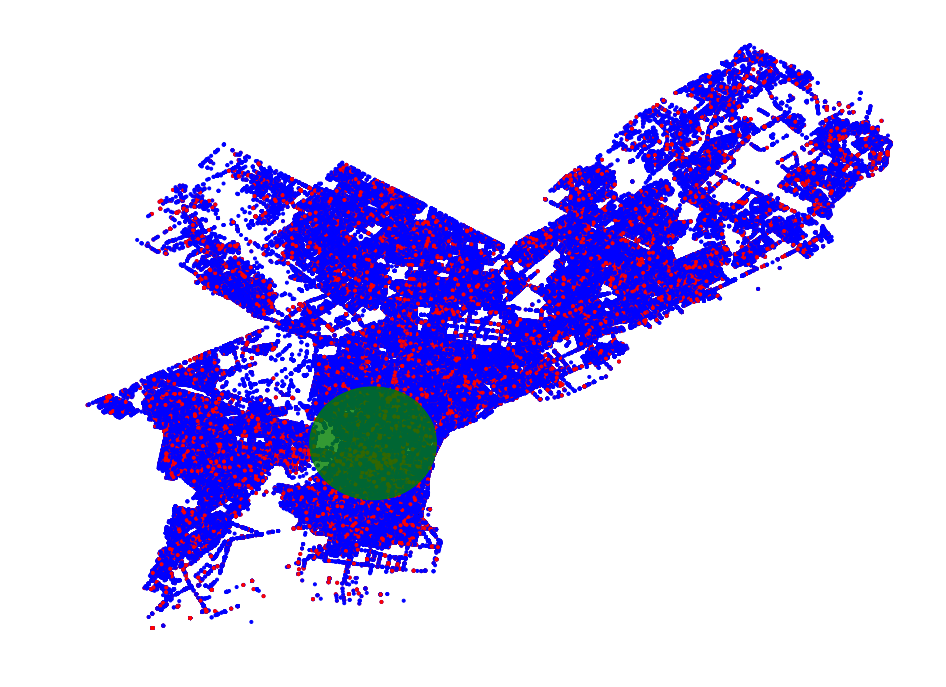
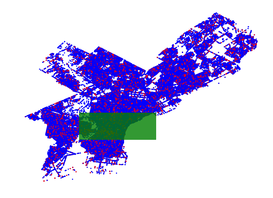
- Philadelphia Crime Data Example
- Region Simplification
- Region Scanning
- Region Scanning Part 2
- Trajectory Approximation
- Trajectory Partial Scanning
- Trajectory Full Scanning
Contents
- Page